Home > Tech Tools > Technical Papers > Capacitor Discharge Current Theory
Abstract—This paper is a detailed explanation of how the current waveform behaves when a capacitor is discharged through a resistor and an inductor creating a series RLC circuit. There are several natural response cases that can occur depending on the values of the parameters in the circuit such as overdamped, underdamped and critically damped response. What this paper will focus on is a way of determining the peak discharge current achieved in the circuit. Traditionally we believe that we can use Ohm’s Law to find the peak current but this is not true in every case.
I. Introduction
The concept behind this paper relates back to perhaps one of the simplest circuits in electronics engineering consisting of the three most common passive components; one resistor, one inductor and one capacitor creating a series connected RLC circuit. We are interested in studying how the current behaves when the capacitor is charged to an initial voltage (Vo) and switched to discharge through the resistor and uncharged inductor (Io=0). Depending on the values of these components one of three types of response can occur. The damping factor will be discussed shortly, and this parameter determines if the response will be underdamped or oscillating, critically damped or overdamped.
The purpose of this paper is to study what happens in the transient state of the discharge cycle and how to approximate the maximum current value achieved by means of mathematical modeling and comparison of experimental results. The peak discharge current is said to be approximated by using Ohm’s Law which does not work in every case. In most overdamped cases this does show useful but as resistance gets smaller and/or inductance gets larger this concept becomes less acceptable.
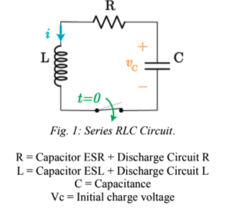
Fig. 1: Series RLC Circuit.
II. Mathematical Modeling of the Circuit
The circuit pictured in Figure 1 can be modeled using Kirchhoff’s Voltage Law summing the voltages of the components and equating to zero. Manipulating the equation using common relationships it can then be put into terms of current and solved as a second order differential equation.
Applying Kirchhoff’s Voltage Law:
VL+VR+VC=0
Relating each expression to current:
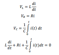
Deriving each equation with respect to t:
![]()
Dividing the equation by L to put it in standard ODE form:
![]()
(1)
We now have the second order differential equation in terms of current that will be solved. Transforming into Laplace Domain to solve the ODE:
![]()
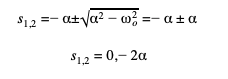
We denote the Neper Frequency as being α=R2L which is a measure of how fast energy is lost in an oscillating system and has a unit of measure of Nepers/second. One other important parameter is the resonant angular frequency which is defined as o=1LC. The equation in the Laplace domain will be rewritten in terms of these two variables: s2+2αs+w2/0=0
The quadratic formula can solve for the s-variable:
![]() (2)
(2)
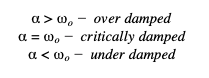
The damping variable was mentioned in the introduction and defined as the determining factor of whether the response type will be underdamped, critically damped or overdamped. We define this variable as:
![]()
Under the following criteria we can distinguish which type of response to expect from our discharge circuit.
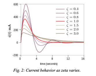
The following image has several overlaying example graphs describing what the current waveform looks like for each case. ζ=1 shows critical damping, <1 shows the oscillatory behavior of the wave in the underdamped region and >1 shows the lower peak amplitude overdamped region.
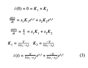
III. Overdamped Response
The overdamped response is what happens when the system returns to equilibrium with no oscillations. This is defined as when ζ>1 or α>O. Solving equation (2) results in both s1 and s2 to be both real and unique roots. When solving a second order differential equation with real, unique roots the general solution is described as:
i(t)=K1es1t+K2es2t
Using initial conditions the variables K1 and K2 can be solved for.
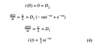
IV. Critically Damped Response
The critically damped response is the borderline between the response oscillating and not oscillating. This is a special case because this means the system is balanced perfectly on the cusp of an oscillatory response. This response is defined as when ζ=1 or α=O. Going back to equation (2) this solution results in two real, non-unique answers. The general solution to the differential equation with two repeating roots is described as:
i(t)=D1te-αt+D2e-αt
Similar to the previous case the initial conditions can be used to solve for the variables D1 and D2.
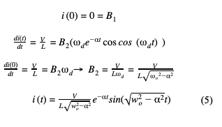
Underdamped Response
The last of the three possible response for the system is the underdamped response which results in an oscillation and continues to oscillate more and take longer to return to equilibrium as gets smaller. When solving equation (2) the roots are now complex as the discriminant is now negative because α<O. The general solution to the differential equation with complex roots is described as:
i(t)=B1e-αtcos cos (wdt)dt +B2e-αtsin(wdt)
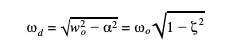
The underdamped response is a sinusoidal signal that is oscillating at a frequency dependent on the angular resonant frequency and the Neper Frequency called the Damped Resonant Frequency. This variable d is defined as:
Using initial conditions the variables B1 and B2 are solved for:
Approximating Peak Current
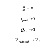
When the peak discharge current is desired, a quick way to find it in most discharge cases is using Ohm’s Law which is calculated using V=IR. This is only correct in a special case where the Neper frequency is much greater than 0. In general this is considered an overdamped response since α>O. Equation (3) will be studied further as the inductance value becomes more insignificant to increase . This will derive the equation that is acceptable to use when the inductance in a discharge circuit is negligible compared to the resistance value. In theory, if the Neper frequency is very large it is acceptable to use an abbreviated model for the overdamped response.
To begin, equation (2) will be solved for as α≫WO.
Now, plugging in s1,2 values into current equation (3) and solving the amplitude first:
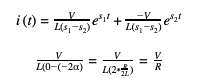
The leading coefficient is found to be V/R. Now the extreme s1,2 values will be evaluated:
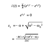
Using L’Hospital’s Rule to evaluate the limit:
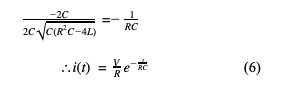
In conclusion, Ohm’s Law has been derived from the general solution equation (3) and proven to be an acceptable approximation for the leading coefficient of the discharge waveform if and only if the inductance of the system approaches zero, or becomes more insignificant.
Why Ohm’s Law Doesn’t Always Work
Section VI discusses and concludes how the circuit will behave as the inductance of a circuit becomes negligible, which we can assume when we are discharging a capacitor through a resistor in the range of ohms and/or an inductor with a very small inductance value. This will make the Neper frequency become much larger than the angular resonant frequency which allows Ohm’s Law to be used to approximate the peak discharge current.
Going more in depth in the behavior of the current waveform, unlike voltage the current waveform does not start at its peak and needs to rise from zero amps. There will always be some delay between t=0 and the instance in which it reaches its peak. It is important to note that from the instant the capacitor starts discharging, it is losing charge and therefore losing voltage since the potential across the capacitor is proportional to the charge stored in it. If the capacitor loses too much charge in the initial ramp up time it will cause the voltage to be significantly lower than the initial value, invalidating Ohm’s Law calculations using the initial charge value. An amended version of the Ohm’s Law model can be derived to give the peak discharge current with inductance and loss of charge in mind.
We can calculate how long it takes the current to ramp to its peak, how much charge was lost in that time, and finally determine the voltage across the capacitor when current reaches its peak. First, evaluate how long it takes for the current to reach its peak by finding the first derivative of equation (3) equating it to zero and finding t.
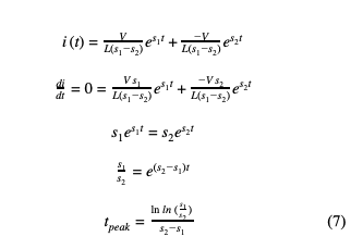
At this point in time, the capacitor has reached its maximum current value. Now using the total electric charge equation, the amount of charge lost during the ramp up time can be found.
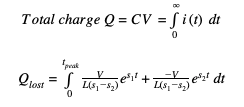
Evaluating the integral,
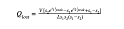
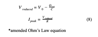
By manipulating the electric charge equation, lost voltage can be found by dividing the lost charge by capacitance. Subtracting the lost voltage from the initial voltage will yield the remaining voltage across the capacitor at the time of peak current. It is at this point the resulting voltage can be divided by resistance to find the peak current value. This results in the general solution for the peak current calculation in overdamped cases when inductance is not neglected.
In conclusion, when there is significant inductance present in a discharge system this will limit the peak current produced by the system. To further explain what happens when inductance approaches zero, the inductor voltage equation can be manipulated and solved for the rate of change of current rise.

Using this equation and the concept of lost charge during the rising period proposed earlier, the theory in equation (6) can be confirmed by letting inductance approach zero. If inductance approaches zero, the slope of the rising current will approach infinity therefore making the rise time infinitely small. With an infinitely small rise time the amount of charge lost will approach zero. Finally, this will result in the voltage at peak current equal to the initial voltage.
VIII. Comparing Calculations with Experiments
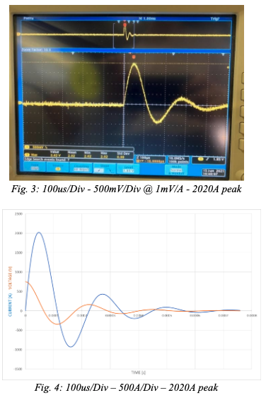
Figure 3 is a photo of experimental results on an oscilloscope when running capacitor discharge pulsing. This image is the results captured with R=0.126Ω L=9.3uH C=130uF and V=750V. The maximum current was found to be 2020A. Figure 4 is a computer simulated model of what the current waveform is predicted to look like when the real-world parameters are set in equation (5). It was found that the maximum current was also 2020A and the waves have the same resonant frequency as expected. This is an example of an underdamped waveform.
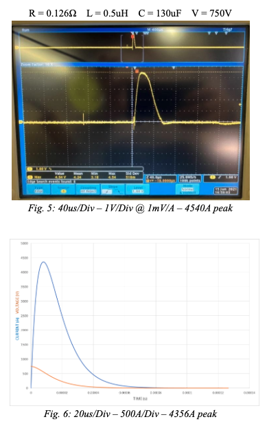
Figure 5 is a photo of experimental results on an oscilloscope, showing the real findings of discharge current achieved with values of R=0.126Ω L=0.5uH C=130uF and V=750V. Figure 6 is the computer simulated waveform of the same parameters in figure 5, calculated with the values as inputs to equation (3) since they are overdamped. The only difference in figures 5,6 compared to in figures 3,4 is the inductance is lower. This will increase the value thus making this an overdamped case.
It is important to notice the new peak current that was achieved by changing the inductance, and the peak time. Figures 3,4 reach peak current of 2020A in 56us while figures 5,6 reach peak current of 4356A in 8us. When the wave requires less time to reach the peak, it results in a higher peak current.
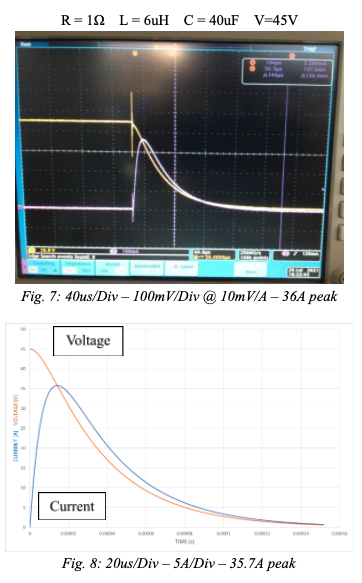
Figure 7 is another example of an overdamped case with values of R=1, L=6uH, C=40uF and V=45V. In this experiment a voltage probe was connected across the capacitor to follow the voltage waveform. In figure 8 the computer model used the input parameters in equation (3). It was found the experimental results and the computer model look remarkably similar and both show a peak current of 35.7A with a rise time of 14us.
IX. Real World Application of Calculations
Now, figure 8 will be focused on and broken down to further analyze the waveform behavior. The R, L, C, and V values are put in equation (3).
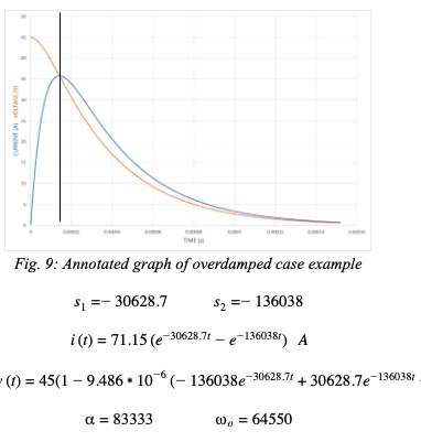
This is an overdamped case so there is no oscillation and inductance is not neglected. is not much greater than o so from the discussion in section 6 equation (6) cannot be used to approximate the peak current. A black line named cursor 1 is placed at the time instant of t=tpeak to focus on what the voltage (orange) and current (blue) waveforms look like at and before this time. An important piece of the graph is to identify where the waves are at t=0 and t=tpeak. Voltage starts at initial charge value of 45V and starts to decline as soon as discharging begins (t=0+). The current waveform starts at 0A at t=0 and ramps up to its peak value of 35.7A at t=tpeak. It can be seen that in the time range of 0≤t≤tpeak the voltage graph had declined by 9.3V. Since the voltage has dropped so much before tpeak this invalidates using Ohm’s Law to approximate the peak current using initial charge voltage. Peak current must be calculated using the mathematics in section 7 and finally using equation (8). Using equation (7) the time it takes for the current to reach its maximum point can be found:
tpeak=14.14 μs
Integrating the model for the current waveform in the range of 0≤t≤tpeak.
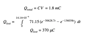
The calculations show that 370 μC was lost during the current rise period. Finally finding the lost voltage:
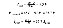
The derived mathematical models found in this report matched the waveforms found experimentally with an oscilloscope and current probe. In addition to this, it has been proven that when inductance is not neglected and is of significance in the system, Ohm’s Law cannot be used to approximate the peak discharge current, in other words we cannot assume that in the time range 0≤t≤tpeak there is no charge lost. Because of the inductance impeding the rise of the discharge current there may be significant charge lost in the ramp time causing the voltage across the capacitor to be lower than expected by time the current reaches its maximum, as seen in figure 7. It is only when inductance can be neglected (α≫o) that it can be assumed negligible charge was lost during the rise time and Ohm’s Law holds.
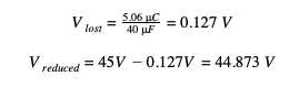
To emphasize this theory, one last experiment is done where a larger resistor was added to the discharge circuit thus making α≫o and allowing Ohm’s Law to be a valid calculation for peak current. The new parameters are R = 57.6Ω L = 55uH and C = 40uF.
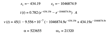
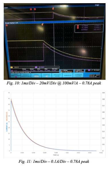
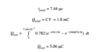
Figure 10 is the oscilloscope output of the experiment. Prior to discharge, voltage is constant at 45 volts and current is at 0 amps and at the time of discharge, the current is very quickly ramped up to peak. Figure 11 shows the computer simulation of this circuit using equation (3) to model the current. After observation it is shown that this simulation is a very close approximation to the real graph. Similar to the last example the charge lost in the time interval 0≤t≤tpeak will be calculated and the voltage loss will be evaluated.
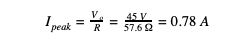
The calculations show that only 5.06 μC was lost during the current ramp up time. Compared to the last example this is only 1.3% of the charge lost previously. Finally finding the lost voltage:
This results in a negligible charge loss during the ramp up period. This concludes that if α≫o there will be a negligible voltage loss in the ramp up time and therefore it is only under this condition that Ohm’s Law can be used to calculate peak current.
X. Conclusions
The objective of this paper was to outline the possibilities of discharge current waveforms and what is happening in the transient state as soon as discharge begins. The three cases that are possible for the response are underdamped (oscillatory), critically damped and overdamped and the response type is determined by the ratio between the Neper frequency and the angular resonant frequency of the system. In the underdamped case the inductance is heavily involved in the system causing the signal to oscillate at a specific frequency called the damped resonant frequency in which the current begins lagging the voltage approaching a shift of 90 degrees.
A major conclusion that have been determined is what is happening to the voltage and current waveforms in the overdamped case between t=0 and the time when the current reaches its peak value, t=tpeak. Since the current equations have been derived, this value can be calculated. During the time interval 0≤t≤tpeak the current starts at zero and is ramping up to its peak value while the voltage starts at initial charge voltage Vo and begins declining. The example on page _ shows the calculations carried out to analytically find the peak current, which was proven to be correct comparing it to real world experiment in figure (7) and computer simulation of the waveforms in figure (8).
A significant conclusion is the current is not at its peak when voltage is at its peak. From the moment discharging begins, current is flowing out of the capacitor therefore it is losing charge. Since voltage across a capacitor is proportional to the charge stored, voltage potential across the capacitor will instantly begin declining as the current is ramping up. Figure 9 shows a clear demonstration of how voltage can be reduced by time the current reaches its peak value. This invalidates the ability to calculate peak discharge current using Ohm’s Law using the initial charge voltage value.
Ohm’s Law is a method that may be used to approximate the peak current in a special case where the Neper Frequency is much greater than the angular resonant frequency (α≫o) which essentially means the ratio of resistance to inductance is very large resulting in a severely overdamped case. On page 3 it is proven that Ohm’s Law does work in this extreme case, but a more generalized approach must be considered when analyzing a circuit that isn’t necessarily severely overdamped. On page 4 it is proven that Ohm’s Law may be used when a reduction in voltage potential is considered. In conclusion the calculations shown in equations (7) and (8) are components of the general solution that can solve for the peak current in any overdamped case.
Tyler Cona
Electronic Concepts, Inc.
Eatontown, United States of America
[email protected]